
Skip to content

search   cart   my account   contact


Expand a hit into a library, and measure every single member.

What the MACS Matchmaker makes possible when the chip position carries the chemical core and the injected sample carries the building block: 64 compounds measured per run, full binding kinetics for each of them, and no sequencing step anywhere in the workflow.

Book a 30-min demo →

Scientific Background

What is encoded library screening?

The usual tag is a barcode, read by sequencing

Encoded library screening is any approach in which each member of a compound library carries a tag that records its chemical identity, so the members can be pooled, screened together, and told apart afterwards.

In a DNA-encoded library (DEL) the tag is a DNA barcode read by next-generation sequencing after selection and washing. What comes back is an enrichment count: how much more often a barcode appeared in the bound fraction than in the input. The count is a ranking signal, not an affinity, and it describes the intended synthesis product rather than the molecule that actually bound.

Here the tag is an address, read by the instrument

The workflow on this page uses the DNA differently. It is not read as a message, it is used as an address. Each chemical core is coupled to its own capture sequence, and DNA-directed immobilization (DDI) places it at one defined position on the sensor chip.

The instrument then reports a binding curve for that position. Identity comes from where the signal appears, not from sequencing what was pulled down. The tag is never amplified, never sequenced, and never decoded.

The Problem

Why hit expansion stalls after the first screen.

A screen tells you that a chemical series is interesting. Turning that into structure-activity relationships means making and measuring the neighbours of the hit, and both halves of that sentence are expensive. The conventional route makes one compound at a time and measures one compound at a time, so cost and calendar scale with the size of the question rather than with its difficulty.

One compound, one synthesis

Expanding a core across a few hundred building blocks conventionally means a few hundred separate syntheses, each purified and characterized before it can be tested at all.

One compound, one measurement

Plate-based affinity work then repeats the same per-compound cost on the analytical side, which is why expansion sets are usually trimmed long before the chemistry runs out of ideas.

Absence of signal teaches nothing

In enrichment-based readouts a compound that does not appear is indistinguishable from one that was never made properly, so the negative half of the matrix, which is where selectivity lives, stays dark.

The useful question is comparative

What a medicinal chemist wants is not one number but a surface: which substitutions this core tolerates, and which cores tolerate this substitution. That question needs the whole matrix, not its top few cells.

The Concept

Put the two diversity axes on two different physical channels.

Axis one, the core, lives in space

A library built by combining n cores with m building blocks has two independent axes. The concept assigns each axis to a different physical channel, so neither has to be decoded from the other.

Every core is coupled to its own DNA capture sequence, so DDI places it at one known position on the chip. Position is identity, and it is fixed before any measurement starts.
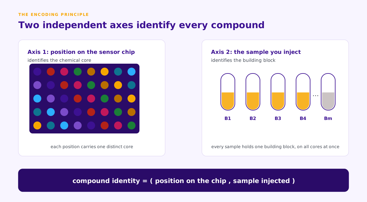
Two independent axes identify every compound: position on the sensor chip encodes the chemical core, the injected sample encodes the building block

Axis two, the building block, lives in the sample

The addressed cores are pooled once, then split into aliquots, and each aliquot is reacted with a single building block. Every aliquot therefore contains all n cores carrying the same building block.

Which aliquot you inject is the second half of the identity. A compound is then specified completely by the pair (position, sample). No barcode has to be sequenced, and no deconvolution step stands between the measurement and the answer.

This is the whole mechanism, and it is deliberately simple. Everything else on this page follows from it.

How It Works

How does the workflow run, step by step?

Four steps take a confirmed core to a fully measured library. Only the third step involves new chemistry, and only the fourth consumes instrument time.
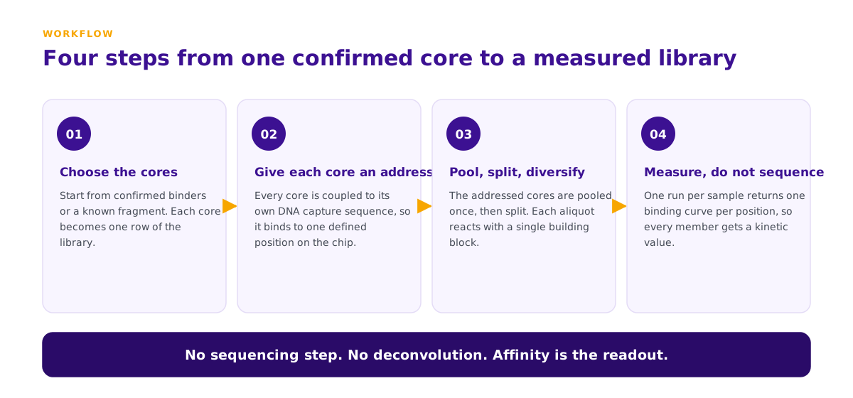
How does the workflow run, step by step?
Protocol details
  • Step 1
    Choose the cores
    Start from confirmed binders, from a fragment with known activity, or from the hit list of a previous screen. Each core becomes one row of the matrix.
  • Step 2
    Give each core an address
    Couple every core to its own DNA capture sequence. The sequence is not a message about the chemistry, it is a postal address that determines where on the chip the core will sit.
  • Step 3
    Pool once, then split and diversify
    Pool the addressed cores, split the pool, and react each aliquot with one building block. This is the step that changes the arithmetic: m reactions produce n times m compounds.
  • Step 4
    Measure instead of sequencing
    Load one aliquot. Each core hybridizes to its own position, so one run returns one binding curve per position, and therefore one affinity value per compound in that aliquot.
64
Compounds measured per run
90 min
Approximate run time
64×
Fewer reactions than one-at-a-time synthesis
0
Sequencing steps required
Instrument Capabilities

What the MACS Matchmaker brings to this workflow.

64
Addressable positions on one sensor chip

DNA-directed immobilization places each core at a predefined position, which is what allows position to serve as identity. This sets the height of the matrix.

1 run
Every position measured at the same time

All positions on the chip are read in the same run under the same conditions, so values within one sample are directly comparable without cross-run normalization.

3 constants
Association, dissociation, and affinity

Each position returns an association rate, a dissociation rate, and an equilibrium dissociation constant KD, so members separate on binding behaviour rather than on a single endpoint value.

pM
Picomolar-range detection

The working range spans picomolar to micromolar affinities, so strong and weak members of the same library stay resolvable in one campaign without pre-sorting by potency.

Crude
Unpurified media are the design case

Focal molography measures in unpurified media. That matters here because the injected sample is a reaction mixture rather than a purified compound.

0
Label or tag added for detection

Detection is label-free and comes from the diffraction of the mologram pattern itself, so nothing has to be attached to the compound in order to see it bind.

Throughput

What a campaign looks like at three sizes.

Conventionally, describing 6,144 compounds would mean 6,144 separate syntheses. In the first row below it means 96. That ratio is the economic argument, and it improves as the chip fills, because the reaction count is the compound count divided by the number of positions. The figures are arithmetic on two published numbers, 64 addressable positions per chip and approximately 90 minutes for a 64-plex run, assuming one run per sample and continuous operation. They are planning scenarios, not measured campaign data.

Samples, one building block eachCompounds measuredChemical reactionsOn one systemOn four in parallel
966,14496about 6 daysabout 1.5 days
38424,576384about 24 daysabout 6 days
96061,440960about 60 daysabout 15 days
The Output

An affinity matrix instead of a hit list.

Every cell carries a measured number

The output is a filled matrix in which every cell is one compound and every cell carries a measured value. That is a different object from a ranked hit list, and it answers different questions.
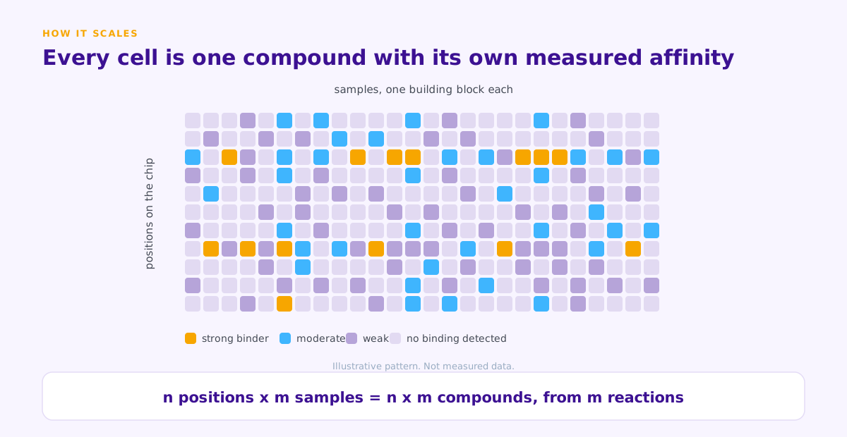
Illustrative affinity matrix: rows are chip positions, columns are samples, every cell is one compound

The empty cells are data too

Because non-binders are measured rather than inferred from absence, the empty regions of the matrix are informative. A core that binds with one building block and a core that binds with forty are immediately distinguishable, which is a selectivity statement that enrichment counts cannot make.

Trends along a row show how one core responds to substitution. Trends down a column show which cores tolerate a given building block. Both readings come out of the same campaign at no extra cost, because the whole matrix was measured rather than sampled.

Comparison

How an affinity readout differs from a sequencing readout.

The two are complementary rather than competing. A selection supplies the cores; this workflow expands them.

PropertyAffinity readout on the sensor chipSequencing readout
Primary signal Association rate, dissociation rate, and KD per compoundEnrichment count from the bound fraction
Identity comes from Position on the chip, fixed before the measurementBarcode sequence, decoded after selection
Non-binders Measured and reported as no binding detectedAbsent from the data, indistinguishable from failed synthesis
Weak binders Quantified within the working range of the instrumentFrequently below the noise of the count statistic
Deconvolution step Not requiredRequired
Reactions per campaign One per building block, acting on all cores at onceOne per compound if members are resynthesized individually
Cost driver Number of building blocksNumber of compounds carried through resynthesis

Want to know what this would look like for your series?

Bring a core and a building-block set, and we will work through the matrix size, the campaign length, and where your chemistry is likely to push back.

Book a 30-min demo →Ask a technical question →

Feasibility

What determines whether this works for your chemistry.

The instrument capabilities above are established. The campaign architecture built on top of them is a concept that has not yet been run end to end, and these are the six factors that decide how well it transfers to a given programme. They are worth working through before a campaign is designed, not after.

Does the chemistry survive pooling?

Every building-block reaction runs on DNA-coupled material in a pooled format and has to tolerate all cores at once. Reactions needing large reagent excess, or leaving poorly soluble products, are the limiting case.

How wide is the building-block set?

Instrument time grows linearly with the number of samples, so the width of the set sets the campaign length. The throughput table above turns that into concrete numbers for three set sizes.

How long is the campaign?

A campaign spanning many consecutive days places the stability requirement on the whole run series rather than on a single measurement. Long campaigns should be planned with that in mind.

How are position effects controlled?

Because identity is positional, the design has to separate a real binding difference from a position artifact. Placing replicate cores at different positions across chips is the direct control.

Is reaction yield tracked separately?

The workflow reports binding, not conversion. A cell showing no binding could be a true non-binder or a failed coupling, so orthogonal quality control on the diversification step stays necessary.

Does the data land in a usable shape?

A matrix-shaped campaign needs a machine-readable result per position and per run rather than a per-chip summary, so the analysis pipeline should be agreed before the first sample is made.

FAQ

Frequently asked questions

Q.How many compounds can one campaign cover?
The height of the matrix is set by the chip, at up to 64 addressable positions. The width is set by how many building-block samples are run, and each sample costs one instrument run. The total is the product of the two, so 96 samples describe 6,144 compounds and 960 samples describe 61,440.
Q.How is this different from conventional DNA-encoded library screening?
Conventional DNA-encoded library screening reads a barcode by sequencing and returns enrichment counts. This workflow uses the DNA as a positional address instead of a message, and returns binding kinetics per compound. The two are complementary: a selection can supply the cores that this workflow then expands.
Q.Can the chemical cores come from a previous DNA-encoded library selection?
Yes, and that is the intended entry point. Hits confirmed by on-DNA validation are exactly the kind of starting material this expansion workflow is designed to consume.
Q.What happens to compounds that do not bind?
They are measured and reported as no binding detected. In this workflow a negative result is a data point rather than a gap, which is what makes selectivity readable across a row of the matrix.
Q.Does the sample have to be purified before injection?
No. Focal molography is designed for unpurified media, which is why a reaction mixture can be injected directly. Residual reagent load still needs checking per chemistry, and that is one of the things worth discussing before a campaign.
Q.Has this workflow been run end to end?
Not yet. The instrument capabilities it relies on are established and published; the campaign architecture built on them is a concept. We would rather state that plainly than imply validation that does not exist.
Q.Can we implement this workflow ourselves?
Yes. It is described here in full and lino Biotech AG holds no patent on it. What we supply is the instrument, the chips, and the support to get the assay running.