

AI designs binders. Screen them at scale.
Measure up to 64 AI-designed binders in parallel on one sensor chip. Go from crude expression to binding kinetics with MACS® Matchmaker, directly from lysate.
Up to 64 Binders in parallel on one sensor chip | 96 Coded pools organized on one plate | Lysate No purification of each design | 2 Capture routes, SpyTag or Twin-Strep-tag |
Turn design libraries into measured priorities.
AI protein design generates candidates for experimental testing. High-throughput binding characterization helps you compare those designs and select the next round. MACS® Matchmaker measures up to 64 binders in parallel, directly from lysate, and links each kinetic result to its design ID to guide selection and subsequent model refinement.
01 / Compute Design a library Generate and prioritize candidate sequences in your AI design workflow. | 02 / Experiment Screen 64 in parallel Measure binding kinetics across coded panels of expressed designs. | 03 / Learn Inform the next round Return binding profiles to your design process and select the next candidates. Model training and sequence generation remain part of your computational workflow. |
Why the bench slows down an AI design campaign.
The candidate list grows with every design round. The way binders are usually characterized does not.
1 Purify every design first Most kinetic methods expect purified protein. For a design library, expression and purification of each candidate becomes the rate-limiting step, long before the first binding curve. | × One interaction at a time Sequential measurements scale linearly with the number of designs. Every additional round of candidates adds the same instrument time again. |
≈ Endpoints hide kinetics Endpoint binding signals and enrichment scores rank designs, but two binders with the same signal can have very different on- and off-rates. The model learns from the coarser number. | ↻ The loop has to close quickly Measured data are only useful to the next design round if they arrive while that round is being planned. A slow characterization step stretches every iteration of the campaign. |
Where conventional methods fall short.
None of these are bad methods. They were built for purified samples or for selection, not for kinetic ranking of large libraries straight from expression.
| Method | Limitation for screening AI-designed binders |
|---|---|
| Surface plasmon resonance (SPR) | Few interactions per cycle, and candidates are usually purified first. For a large design library the sample preparation, not the measurement, sets the pace. |
| Biolayer interferometry (BLI) | Parallel across a plate of tips, but each binder needs its own tip, and crude lysate adds nonspecific background to the refractive signal. |
| High-throughput SPR arrays | High parallelism for antibody panels, but refractive-index sensing still has to be referenced carefully when the sample is a crude matrix. |
| ELISA and plate binding assays | Endpoint readouts. Binders with the same equilibrium signal but different kinetics look the same. |
| Display selection (phage, yeast) | Ranks clones by enrichment under selection conditions, not by measured kon, koff and KD. |
One pool. Up to 64 binder profiles.
Express your AI-designed candidates, assign DNA codes and pool up to 64 binders. DNA-directed immobilization (DDI) sorts each binder onto its assigned sensor spot.
01 / Express Start with lysate 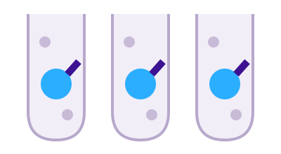 Express each AI-designed binder separately with a SpyTag or Twin-Strep-tag. Retain its design ID throughout the workflow. | 02 / Code Assign a DNA code 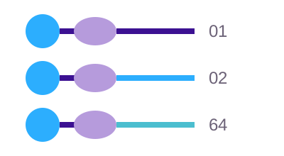 Add a different coded capture adapter to each lysate, with binder in excess over adapter. | 03 / Pool Pool up to 64 binders 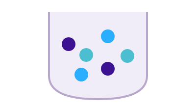 Combine coded lysates into one well. Organize additional pools across a 96-well plate for larger design libraries. | 04 / Measure Measure in parallel 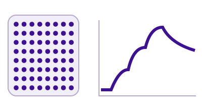 Self-sort the pool on the chip, then measure target binding across up to 64 candidates in parallel. Regenerate and load the next pool. The curve illustrates single-cycle kinetics, it is not experimental data. |
Scale beyond a single panel. Combine 64-plex measurements with a 96-well pooling workflow to plan larger AI design campaigns. Measure each pool sequentially against the target. | 96×64=6,144 Nominal design capacity: 96 pools × 64 positions, before controls and replicates. Actual throughput depends on the assay and regeneration performance. |
Choose the tag that fits your construct.
The capture adapter connects your tagged binder to its DNA code. Both routes feed into the same split-and-pool workflow, and both adapters are available in the webshop, pre-conjugated to the DNA code of your choice.
SpyTag + Oligo Adapter SpyCatcher
SpyTag on the binder reacts with the Oligo Adapter SpyCatcher to form a covalent bond. The adapter's DNA code provides the address on the sensor chip.
Twin-Strep-tag® + Oligo Adapter Strep-Tactin® XT
Twin-Strep-tag on the binder binds the Oligo Adapter Strep-Tactin® XT. This capture interaction attaches the binder to its DNA address.
Protocol details.
What a screening campaign is built from, on the instrument and the consumables of the standard MACS Matchmaker workflow.
| Parameter | Value |
|---|---|
| Sample | Crude lysate of separately expressed binders. Tag accessibility, expression level and sample compatibility need to be checked for your constructs. |
| Capture tags | SpyTag (covalent, Oligo Adapter SpyCatcher) or Twin-Strep-tag (affinity, Oligo Adapter Strep-Tactin® XT). |
| Immobilization | DNA-directed immobilization (DDI). The DNA code on each adapter assigns the binder to its sensor spot. |
| Adapter ratio | Binder in excess over adapter, which favors loading of the coded adapters before pooling. The suitable ratio depends on expression level and capture efficiency. |
| Plex per chip | Up to 64 binders measured in parallel. Controls and replicates reduce the number of unique candidates. |
| Pools | Organized across a 96-well plate and measured sequentially against the target, with regeneration between pools. |
| Nominal design capacity | 96 pools × 64 positions = 6,144, before controls and replicates. Actual throughput depends on the assay and regeneration performance. |
| Readout | kon, koff and KD where the data support a kinetic model, from a target concentration series. |
Rank AI designs by measured binding.
kon How fast does it bind? Compare association rates to see how quickly each binder engages the target. | koff How long does it stay? Compare dissociation rates to distinguish interactions with different complex lifetimes. | KD How strong is the interaction? Combine association and dissociation rates to estimate affinity under an appropriate binding model. |
Lysate No purification step Tagged binders are captured directly from the expression lysate, so every design reaches the chip without its own purification. | Design ID Data that map back Each DNA code maps to one design ID, so every kinetic result returns to the right sequence in your model. | Regenerate The next pool on the same chip Regenerate the surface and load the next pool, so a plate of pools runs as one campaign. |
Binding is round one. Developability is round two.
A design that binds its target can still fail later through nonspecific binding or poor behavior in plasma. Take your shortlisted binders into developability panels that run on the same instrument, directly in complex samples.
Developability Polyreactivity Panel Flag nonspecific binding and other developability liabilities before a design moves forward. Open the Polyreactivity Panel | ADME Plasma Protein Binding See how your lead designs behave in undiluted human plasma. Open Plasma Protein Binding | Service Developability Data Service Send your shortlist and receive a developability package run by our scientists. Open the Developability Data Service |
Before you build your panel.
More from the same platform.
The same DNA-coded capture and the same instrument, applied to neighboring questions.
Small molecules Encoded Library Screening A related 64-plex workflow for small molecules: expand a hit into a library and measure every member. Open Encoded Library Screening | Consumables Oligo Adapters DNA-coded adapters that load each ligand onto its assigned sensor spot by DNA-directed immobilization. Open the Oligo Adapters | Service Custom Measurement Service Send samples, receive kinetics. No instrument required. Open the Custom Measurement Service |
Your next AI design library. Ready for experimental screening.
Bring your target and your candidate count. We help you plan a 64-plex screening workflow with SpyTag or Twin-Strep-tag capture.